Not Another Post about Weather Data in R

Purpose

As part of our conservation program at the University Museum, we collect environmental data in the collections storage rooms. One of the things I want to accomplish is to relate environmental data collected inside the building to contemporaneous environmental conditions outside the building. We’re in the arid high desert. We experience hot summers and monsoon conditions. We also experience large temperature fluctuations throughout the day. I’d like to get towards understanding how these patterns outside are impacting changes inside the building.

The Museum’s loggers record temperature, relative humidity, and dew point every 10 seconds. In terms of conservation, we are concerned about keeping parameters within target thresholds, and we want to be particularly aware of high amplitude fluctuations. In comparing to conditions outside the building, we also want data that includes multiple readings throughout the day.

What Worked

In working towards what I was looking for, I tried many things that didn’t work. In this post, what works is up front while some of the stuff that didn’t work is listed at the end (Section 3).

In finding a workflow that met my needs, I got key inspiration from the Data Whisperer’s video on How to Load Weather Data Directly Into R. Their solution used the riem library which scrapes from the Iowa State University, Iowa Environment Mesonet (IEM), Automated Surface Observing System (ASOS). This archive is “considered to be the flagship automated observing network.”

ASOS stations are located at airports. The closest station is at Las Cruces International Airport which is 15 km from the University Museum. That’ll do.

To get the data one wants, it is necessary to know the appropriate station identifier which can be looked up by network. The New Mexico network it is NM_ASOS, and the Las Cruces station is LRU. I found the name with View(riem_networks()) which gave me a searchable list of networks. Using that, I got a searchable list of stations within the network with View(riem_stations(network = "NM_ASOS")).

LRU offers 20 minute interval data. It is worth noting, that some stations offer 1 minute observations. Unfortunately, there aren’t any for Las Cruces. However, there are two nearby stations that do. El Paso International Airport, TX (ELP) is 63 km from the museum and the Deming Municipal Airport, NM (DMN) is 90 km from the museum.

These two stations are far enough away with sufficiently different local conditions, that I’ll take the coarser resolution of Las Cruces in lieu of the finer resolution data from more distant stations. For the future, it would be interesting to think about interpolating finer resolution data for Las Cruces by using data from El Paso and Deming. Probably not that complicated but for another day.

For the current purpose, let’s load the data and make a plot…

First call the necessary libraries.

library(dplyr)
library(riem)
library(xts)
library(dygraphs)

Then request data and evaluate results (Table 1).

# Request data
measures <-
  riem_measures(station = "LRU",
                date_start = "2020-01-01",
                date_end = "2023-07-16")

# Check data structure
head(measures) |> 
  rmarkdown::paged_table()

Table 1: The first rows of station LRU

To use the dygraphs library, the data need to be converted to a time series. I use xts to create objects for temperature and relative humidity which are variables recorded at the museum. I also added precipitation just to check it out. Once as a time series object, I called the dygraph function and gave it some minimal styling.

# Create time series for each column of interest
las_cruces_temperature <- xts(measures$tmpf, measures$valid)
las_cruces_rh <- xts(measures$relh, measures$valid)
las_cruces_precip <- xts(measures$p01i, measures$valid)


# Bind individual time series
las_cruces <- cbind(las_cruces_temperature, las_cruces_rh)


# Construct graph
dygraph(las_cruces) |> 
  dyRangeSelector() |> 
  dySeries("las_cruces_temperature", label = "Temperature") |> 
  dySeries("las_cruces_rh", label = "RH")

Figure 1: Graph showing temperature and relative humidity for the LRU

This graph is roughly similar to how I visualize environmental data we log inside the museum. I think this is an initial step towards comparing the data. I think the next step would be to look temperature correlation. If there is a tight relationship, then we should be able to more closely predict conditions inside the building based on conditions outside.

library(ggplot2)

In addition to a time series, we can also construct a scatterplot from the original data frame. We’ll plot temperature as the independent variable and relative humidity as the dependent (Figure 2).

It would be nice to color the points by season. For that, we can use the time2season function from the hydroTSM library.

library(hydroTSM)

Add a new season column.

measures$season <- time2season(measures$valid, out.fmt = "seasons")

ggplot(measures, aes(x=tmpf, y = relh, color=season)) +
  geom_point(size = .7, alpha = .1)+
  guides(colour = guide_legend(override.aes = list(size=2, alpha=.7))) # Override aes for legend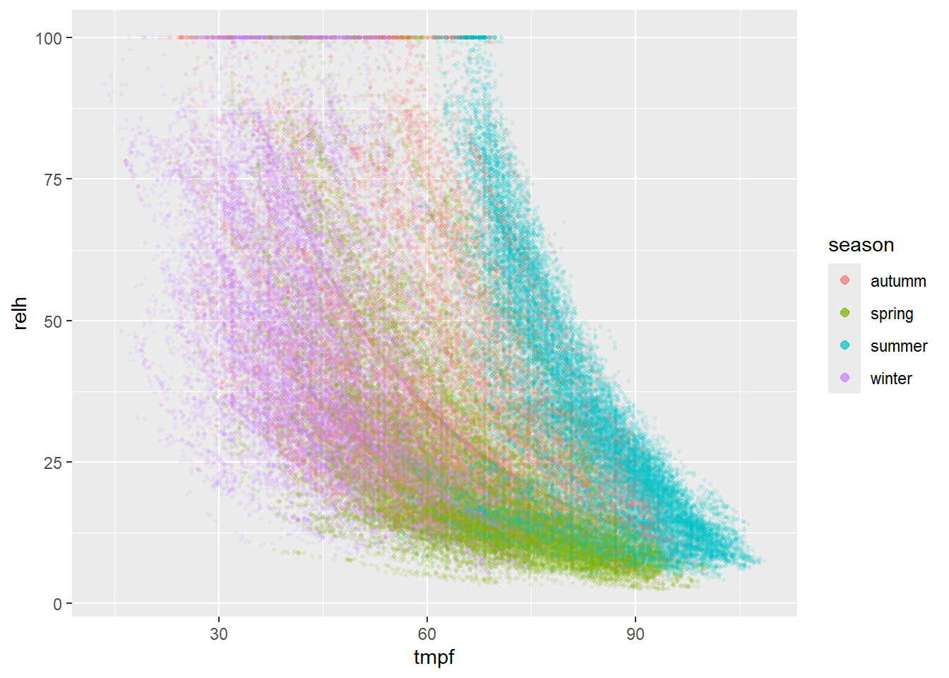

Figure 2: Biplot of humidity against temperature

I thought it would be fun to correlate temperature and relative humidity. My first attempt returned NA indicating that there are missing values in the data.

cor(measures$tmpf, measures$relh)

[1] NA

This SO question helped me understand which argument to use when there are NA. So trying this again:

cor(measures$tmpf, measures$relh, use = "complete.obs")

[1] -0.5164813

Looks like there is a weak negative correlation. Looking at Figure 2 it seems like the correlation grows stronger as the temperature is higher.

Correlation when the temperature is greater than 60 °F:

cor(measures[ measures$tmpf>=60, ]$tmpf, measures[ measures$tmpf>=60, ]$relh, use = "complete.obs")

[1] -0.3752615

Correlation when the temperature is below 60 °F:

cor(measures[ measures$tmpf<=60, ]$tmpf, measures[ measures$tmpf<=60, ]$relh, use = "complete.obs")

[1] -0.3876381

Seems like they are similar, good to check.

What Didn’t Work or I Didn’t Understand

I’m tracking some of the things that didn’t work just as a matter of logging notes. I’d really like to get data directly from NOAA, but it was really confusing.

Other Tutorials

I didn’t want to load a local CSV, I wanted to pull the data directly from the source. The weatherData library is designed to do this, but does not work with R version 4.2.1 (2022-06-23 ucrt) which I am presently running. If weatherData is updated, I would definitely check it out. There’s also rnoaa, but it is being archived because NOAA’s API structure and endpoints changed. Here again, something to watch for. As part of Pat Schloss Climate Change Data Visualization series, he describes Scraping weather data from the internet with R and the tidyverse. That is a useful tutorial, but the data weren’t exactly what I was looking for. I tried Michael Minn’s Weather Data Analysis in R, but had a hard time finding the station I was looking for. I went to NMSU and requested data from the Main Campus station for the period of interest. I had to resort to downloading a CSV. Unfortunately, I was only able to get daily summaries. I was looking for a more frequent sampling interval to track daily changes.

Government data

I’ve got to be honest, the National Oceanic and Atmospheric Administration’s (NOAA) National Centers for Environmental Information (NCEI), Climate Data Online (CDO) confused me. I never did find what I was looking for, but I did get close.

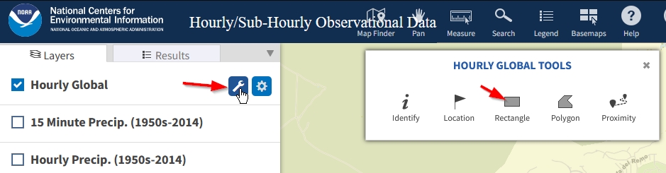
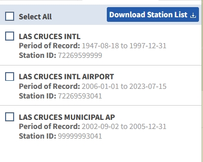
I stumbled around the confusing labyrinth of choices that is the NOAA website and finally found sort of what I was looking for. Using the the map interface for hourly data, I found the Las Cruces airport station. To evoke the search tool, click on the wrench, then draw a box around the stations plotted on the map (Figure 3). This brings up a list of stations (Figure 4).

Figure 3: Spatial search

Figure 4: Spatial search result

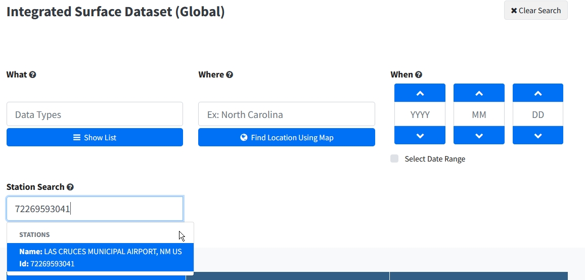
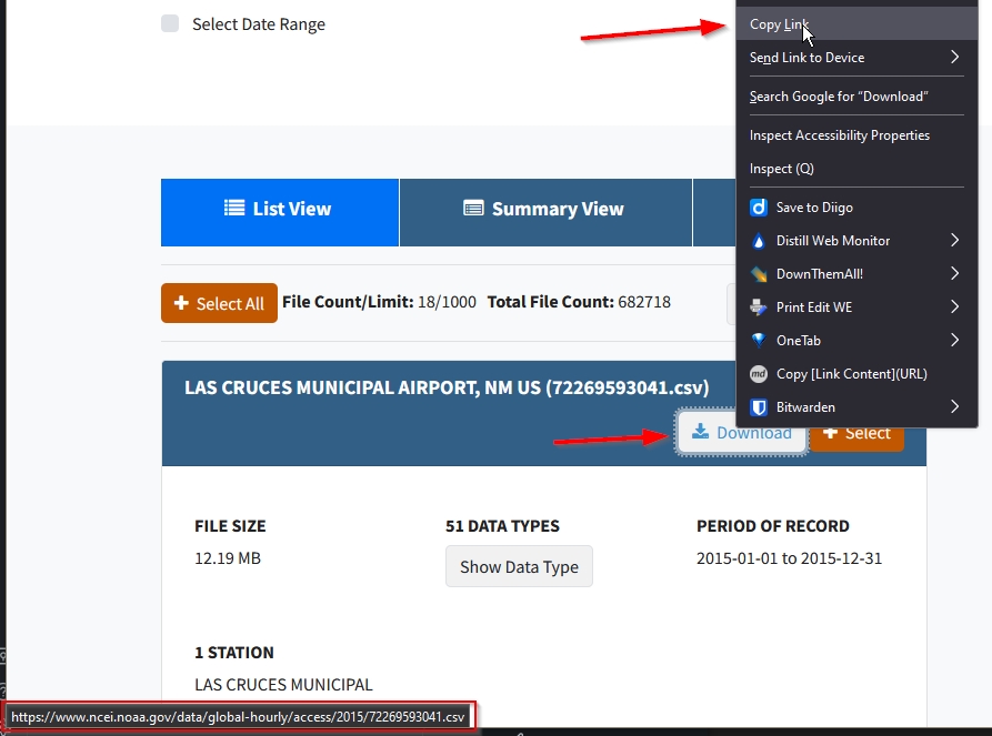
With a station number in hand, I went over to the Data Search page and entered the station id into the Station Search field (Figure 5). This returned data for a range of years, but they weren’t in order. However, I hovered the mouse pointer over a download button and noticed that it returned a result URL with a very logical path. I right clicked over the download button and and selected Copy Link (Figure 6).

Figure 5: Enter station id into Station Search field

Figure 6: Station results hovering over download button. Note the URL showing in the bottom left hand corner.

From there, I created two additional URL’s to cover the needed date range.

URL’s for the years and station of interest

• https://www.ncei.noaa.gov/data/global-hourly/access/2021/72269593041.csv
• https://www.ncei.noaa.gov/data/global-hourly/access/2022/72269593041.csv
• https://www.ncei.noaa.gov/data/global-hourly/access/2023/72269593041.csv

With these, I used readr::read_csv to pull the data from the URL into a dataframe. My plan was to use rbind to bring them together, but each has different numbers of rows. I discovered this when rbind failed. Given this, I’ll just isolate the variables of interest.

df22 <- readr::read_csv("https://www.ncei.noaa.gov/data/global-hourly/access/2022/72269593041.csv")
df23 <- readr::read_csv("https://www.ncei.noaa.gov/data/global-hourly/access/2023/72269593041.csv")
df21 <- readr::read_csv("https://www.ncei.noaa.gov/data/global-hourly/access/2021/72269593041.csv")

ncol(df21)

[1] 50

ncol(df22)

[1] 55

ncol(df23)

[1] 53

Checking the readme for the data helps. I found it at:

https://www.ncei.noaa.gov/data/global-summary-of-the-day/doc/readme.txt

The readme showed that temperature (TEMP) and dew point (DEWP) were present. However, the readme file does not contain the word humidity so the data lack relative humidity data. Bummer… However, all is not lost because dew point and temperature it is possible to calculate relative humidity.

Field names from data set readme.

• STATION - Station Number
• DATE - Given in mm/dd/yyyy format
• LATITUDE - Given in decimated degrees (Southern Hemisphere values are negative)
• LONGITUDE - Given in decimated degrees (Western Hemisphere values are negative)
• TEMP - Mean temperature (.1 Fahrenheit)
• DEWP - Mean dew point (.1 Fahrenheit)
• SLP - Mean sea level pressure (.1 mb)
• STP - Mean station pressure (.1 mb)
• VISIB - Mean visibility (.1 miles)
• WDSP – Mean wind speed (.1 knots)
• MXSPD - Maximum sustained wind speed (.1 knots)
• GUST - Maximum wind gust (.1 knots)
• MAX - Maximum temperature (.1 Fahrenheit)
• MIN - Minimum temperature (.1 Fahrenheit)
• PRCP - Precipitation amount (.01 inches)
• SNDP - Snow depth (.1 inches)
• FRSHTT – Indicator for occurrence of:
  • Fog
    
  • Rain or Drizzle
  • Snow or Ice Pellets
  • Hail
  • Thunder
  • Tornado/Funnel Cloud

We will take: STATION, DATE, TMP, DEW

df21 <- select(df21, STATION, DATE, TMP, DEW)
df22 <- dplyr::select(df22, STATION, DATE, TMP, DEW)
df23 <- dplyr::select(df23, STATION, DATE, TMP, DEW)

df <- rbind(df21, df22, df23)

df$TMP[1:5]

[1] "+0060,1" "+0052,1" "+0039,1" "+0032,1" "+0014,1"

Unfortunately, those aren’t useful numbers. I don’t know what the heck is going on. These values look nothing like the sample data that are located in the documentation.