Scraping Wikipedia Table: Genocides

Introduction

Recently I read an article in Coding the Past about using ChatGPT to wrangle Wikipedia tables into a format usable in R. I tried the method, but found it didn’t work well with tables that had blank cells. Many wikipedia tables have blank cells, so this is likely to be a common issue. Following a post on pipe dreams, I turned instead to using rvest for scraping wikipedia table data. In my experience, scraping the data is a much better option than messing around with ChatGPT.

I selected the list of genocides as the table to retrieve.

library(ggplot2)

Select the table and scrape the object

url <- "https://en.wikipedia.org/wiki/List_of_genocides"

url_bow <- polite::bow(url)

Inspect the page and look for HTML called table.wikitable.

ind_html <-
  polite::scrape(url_bow) |>   # scrape web page
  rvest::html_nodes("table.wikitable") |>  # pull out specific table
  rvest::html_table(fill = TRUE) 

The rvest function returns a list of one item, so we need to index the first item in the list to get the data frame. We do so using the double square bracket [[]] index operator which returns an object of the class of item that is contained in the list.

ind_html[[1]] |>
  head() 

Event	Location	Period	Period	Estimated killings	Estimated killings	Proportion of group killed
Event	Location	From	To	Lowest	Highest	Proportion of group killed
Rohingya genocide[N 1]	Rakhine StateMyanmar	2016	Present	9,000–13,700[9]	43,000[10]	Before the 2015 Rohingya refugee crisis and the military crackdown in 2016 and 2017, the Rohingya population in Myanmar was around 1.0 to 1.3 million, chiefly in the northern Rakhine townships, which were 80–98% Rohingya. Since 2015, over 900,000 Rohingya refugees have fled to south-eastern Bangladesh alone, and more to other surrounding countries, and major Muslim nations. More than 100,000 Rohingyas in Myanmar are confined in camps for internally displaced persons.
Iraqi Turkmen genocide[N 2]	Islamic State-controlled territory in northern Iraq	2014	2017	3,500	8,400
Genocide of Yazidis by the Islamic State[N 3]	Islamic State-controlled territory in northern Iraq and Syria	2014	2019	2,100[18]	5,000[19]
Darfur genocide[N 4]	Darfur, Sudan	2003	Present	98,000[22]	500,000[23]
Effacer le tableau[N 5]	North Kivu, Democratic Republic of the Congo	2002	2003	60,000[26][24]	70,000[26]	40% of the Eastern Congo’s Pygmy population killed[N 6]

Remove footnotes and commas and convert strings into numbers

This worked well, but there are still lingering characters from footnotes. We want to remove the brackets and the numbers inside them, but leave the rest of the text. These can be removed with regular expressions…so time to turn to StackOverflow. We’ll start with an isolated example, ensure that works properly, and then attempt to apply it to the entire data frame.

test <- "2,100[17]"

To do this, we’ll need to use the double escape //.

test2 <- gsub("\\[([^]]+)\\]", "",test)
test2

[1] "2,100"

lapply(ind_html[[1]], function(x) gsub("\\[([^]]+)\\]", "",x)) |>
  as.data.frame() |> 
  head()

Event	Location	Period	Period.1	Estimated.killings	Estimated.killings.1	Proportion.of.group.killed
Event	Location	From	To	Lowest	Highest	Proportion of group killed
Rohingya genocide	Rakhine StateMyanmar	2016	Present	9,000–13,700	43,000	Before the 2015 Rohingya refugee crisis and the military crackdown in 2016 and 2017, the Rohingya population in Myanmar was around 1.0 to 1.3 million, chiefly in the northern Rakhine townships, which were 80–98% Rohingya. Since 2015, over 900,000 Rohingya refugees have fled to south-eastern Bangladesh alone, and more to other surrounding countries, and major Muslim nations. More than 100,000 Rohingyas in Myanmar are confined in camps for internally displaced persons.
Iraqi Turkmen genocide	Islamic State-controlled territory in northern Iraq	2014	2017	3,500	8,400
Genocide of Yazidis by the Islamic State	Islamic State-controlled territory in northern Iraq and Syria	2014	2019	2,100	5,000
Darfur genocide	Darfur, Sudan	2003	Present	98,000	500,000
Effacer le tableau	North Kivu, Democratic Republic of the Congo	2002	2003	60,000	70,000	40% of the Eastern Congo’s Pygmy population killed

So far so good, the footnote characters are gone, so lets save this as a dataframe. However, there is a bit more work to do before this can be graphed.

df <- lapply(ind_html[[1]], function(x) gsub("\\[([^]]+)\\]", "",x)) |> 
  as.data.frame()  

Strings that contain a comma are coerced to NA and this isn’t useful. So the commas need to be removed

as.numeric(test2)

[1] NA

We can use gsub() to remove the , and then convert to numeric.

gsub(",", "", test2) |> 
  as.numeric()

[1] 2100

We need to remove the commas from any column that has numbers, but we want to keep commas in columns that are text. The low end estimate column has some ranges that are separated by a - so we would want to either take the numbers before or after this character. Since these are supposed to be low estimates, we’ll take numbers before and remove everything from the - to the end.

df$Estimated.killings <- as.numeric(gsub(",", "", df$Estimated.killings))

sample(df$Estimated.killings, 20)

 [1]  200000  248000  130000    2100   10000  480000  491000   80000  300000
[10]   34000    3500   50000  600000  111091   50000   60000   34000   83000
[19] 4204000      NA

Plotting the table: sorted bar chart and long x values

We can plot loss of life by event using a bar chart.

The plot presents two fairly common challenges.

1. Some of the label text is very long. As described in this post and the documentation, we can use the scale_x_discrete() function with the label_wrap_gen() argument.

2. The numbers are very large and would be better represented as an abbreviation. This can be achieved with the scales() package using the label_number() argument scale_cut with a value of cut_short_scale(). The documentation and a tidyverse blog post provide some other options.

df |> 
  dplyr::filter(!is.na(Estimated.killings)) |>  # remove NA values
  ggplot(aes(x = reorder(Event,Estimated.killings), y = Estimated.killings)) +
    geom_bar(stat = "identity", position=position_dodge(.5)) +
    scale_x_discrete(labels = label_wrap_gen(50))+
    scale_y_continuous(labels = scales::label_number(scale_cut = scales::cut_short_scale())) +
    coord_flip()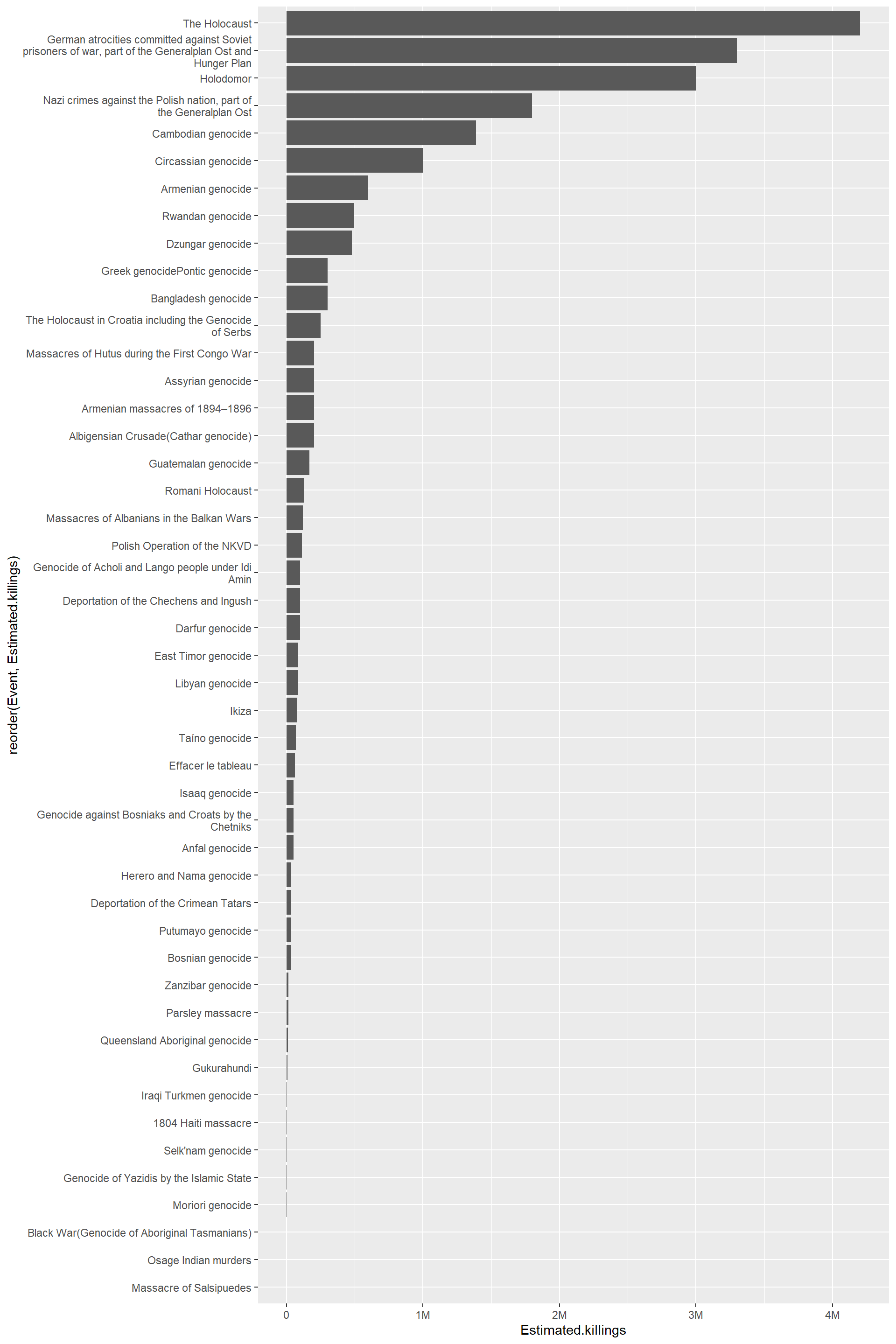

Just noting that if we reorder based on location, the reorder function does not work properly (I did this). The issue is that there three locations where more than one genocide is listed on the table.

df |> dplyr::count(Location) |> dplyr::arrange(n) |> tail()

	Location	n
42	Ukraine and the heavily Ukrainian-populated northern Kuban, in the Soviet Union	1
43	Uruguay	1
44	Van Diemen’s Land (now Australia)	1
45	Zanzibar (now part of Tanzania)	1
46	Ottoman Empire (now Turkey, Syria and Iraq)	2
47	German-occupied Europe	3

According to this answer over at the RStudio forums, ggplot sums the values within each of these locations. In the case of German-occupied Europe, there are three genocides summed so the value is exceptionally large. However, Ottoman Empire (now Turkey, Syria and Iraq) is also not displaying properly. It just isn’t as easy to spot.

df |> 
  dplyr::filter(!is.na(Estimated.killings)) |>  # remove NA values
  ggplot(aes(x = reorder(Location,Estimated.killings), y = Estimated.killings)) +
    geom_bar(stat = "identity") +
    scale_y_continuous(labels = scales::label_number(scale_cut = scales::cut_short_scale()))+
    scale_x_discrete(labels = label_wrap_gen(40))+
    coord_flip()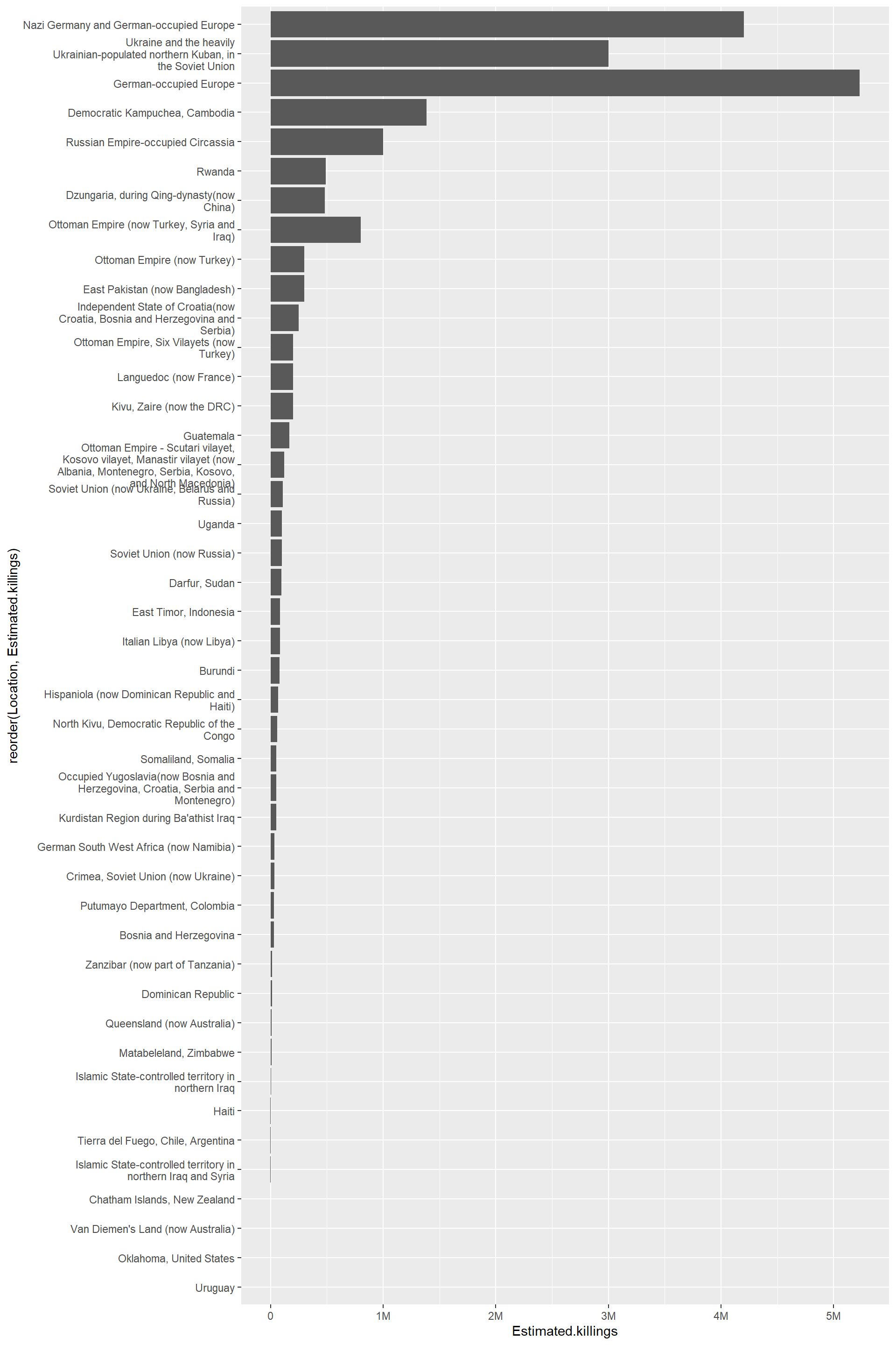

• python - How can I remove text within parentheses with a regex? - Stack Overflow
• regex - Regular expression to extract text between square brackets - Stack Overflow
• r - How do I deal with special characters like ^$.?*|+()[{ in my regex? - Stack Overflow
• r - Applying gsub to various columns - Stack Overflow Specifically, this answer worked in the present case.